


Cuprins
Sparklines first appeared in Excel 2010 and have been growing in popularity ever since. Although sparklines are very similar to thumbnail charts, they are not the same thing and have slightly different purposes. In this tutorial, we’ll introduce you to sparklines and show you how to use them in an Excel workbook.
There are times when you need to analyze and explore a dependency in an Excel dataset without creating a complete chart. Sparklines are small charts that fit into a single cell. Due to their compactness, you can include several sparklines at once in one workbook.
In some sources, sparklines are called information lines.
Types of sparklines
There are three types of sparklines in Excel: Sparkline Graph, Sparkline Histogram, and Sparkline Win/Loss. Sparkline Plot and Sparkline Histogram work in the same way as normal plots and histograms. A win/loss sparkline is similar to a standard histogram, but it does not display the magnitude of the value, but whether it is positive or negative. All three types of sparklines can display markers at important locations, such as highs and lows, making them very easy to read.
What are sparklines used for?
Sparklines in Excel have a number of advantages over regular charts. Imagine you have a table with 1000 rows. A standard chart would plot 1000 data series, i.e. one row for each line. I think it is not difficult to guess that it will be difficult to find anything on such a diagram. It is much more efficient to create a separate sparkline for each row in an Excel table, which will be located next to the source data, allowing you to visually see the relationship and trend separately for each row.
In the figure below, you can see a rather cumbersome graph in which it is difficult to make out anything. Sparklines, on the other hand, allow you to clearly track the sales of each sales representative.
In addition, sparklines are beneficial when you need a simple overview of the data and there is no need to use bulky charts with many properties and tools. If you wish, you can use both regular graphs and sparklines for the same data.
Creating Sparklines in Excel
As a rule, one sparkline is built for each data series, but if you wish, you can create any number of sparklines and place them where necessary. The easiest way to create the first sparkline is on the topmost row of data, and then use the autofill marker to copy it to all the remaining rows. In the following example, we’ll create a sparkline chart to visualize the sales dynamics for each sales rep over a specific period of time.
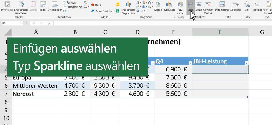
- Select the cells that will serve as input for the first sparkline. We will choose the range B2:G2.
- Faceți clic pe fila Insera and select the desired type of sparkline. For example, a sparkline chart.
- Va apărea o casetă de dialog Creating Sparklines. Using the mouse, select the cell to place the sparkline, and then click OK. In our case, we will select cell H2, the link to the cell will appear in the field Location range.
- The sparkline will appear in the selected cell.
- Click and hold the left mouse button and drag the autofill handle to copy the sparkline to adjacent cells.
- Sparklines will appear in all rows of the table. The following figure shows how the sparklines visualize the sales trends for each sales rep over a six-month period.
Change the appearance of sparklines
Adjusting the appearance of a sparkline is quite simple. Excel offers a range of tools for this purpose. You can customize the display of markers, set the color, change the type and style of the sparkline, and much more.
Marker display
You can focus on certain areas of the sparkline graph using markers or points, thereby increasing its informativeness. For example, on a sparkline with many large and small values, it is very difficult to understand which one is the maximum and which is the minimum. With options enabled Punct maxim и Punct minim make it much easier.
- Select the sparklines you want to change. If they are grouped in neighboring cells, then it is enough to select any of them to select the entire group at once.
- În fila Avansat Constructor în grupul de comandă Spectacol enable options Punct maxim и Punct minim.
- The appearance of sparklines will be updated.
Schimbarea stilului
- Select the sparklines you want to change.
- În fila Avansat Constructor click on the dropdown arrow to see even more styles.
- Select the desired style.
- The appearance of sparklines will be updated.
Type change
- Select the sparklines you want to change.
- În fila Avansat Constructor select the type of sparkline you want. For example, grafic de bare.
- The appearance of sparklines will be updated.
Each type of sparkline is designed for specific purposes. For example, a win/loss sparkline is more suitable for data where there are positive or negative values (for example, net income).
Changing the display range
By default, each sparkline in Excel is scaled to match the maximum and minimum values of its source data. The maximum value is at the top of the cell, and the minimum is at the bottom. Unfortunately, this does not show the magnitude of the value when compared to other sparklines. Excel allows you to change the appearance of sparklines so that they can be compared to each other.
How to change the display range
- Select the sparklines you want to change.
- În fila Avansat Constructor alege echipa Axă. Va apărea un meniu derulant.
- In the parameters for the maximum and minimum values along the vertical axis, enable the option Fixed for all sparklines.
- Sparklines will be updated. Now they can be used to compare sales between sales representatives.