


If you’re looking for a modern way to visualize data, take a look at the Excel watch face chart. The dial chart is literally designed to decorate the dashboard, and because of its resemblance to a car speedometer, it is also called a speedometer chart.
The clock face chart is great for showing performance levels and milestones.
Pas cu pas:
- Create a column in the table Forma (which means the dial) and in its first cell we enter the value 180. Then we enter the range of data showing the effectiveness, starting with negative values. These values must be a fraction of 180. If the original data is expressed as a percentage, then it can be converted to absolute values by multiplying by 180 and dividing by 100.
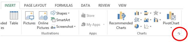
- Highlight a column Forma and create a donut chart. To do this, on the tab Insera (Inserați) în secțiune diagrame (Charts) click the small arrow in the lower right corner (shown in the figure below).

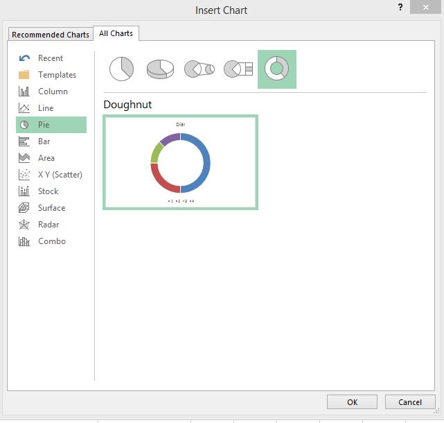
- Se va deschide o casetă de dialog Introduceți o diagramă (Insert chart). Open a tab Toate diagramele (All Charts) and in the menu on the left, click Circular (Pie). Select from the suggested subtypes Inel (Doughnut) chart and click OK.
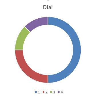
- The chart will appear on the sheet. In order for it to look like a real dial, you will need to slightly change its appearance.
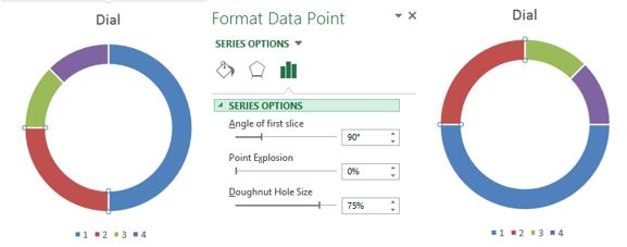
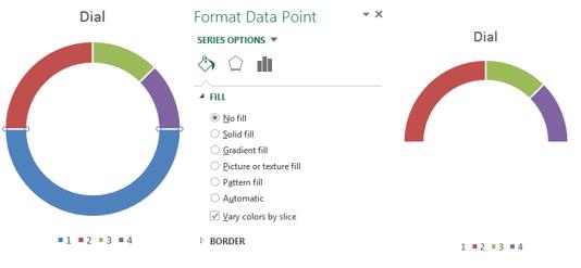
- Selectați punctul 2 in data series Forma. In panel Formatul punctului de date (Format Data Point) change the parameter Unghiul de rotație al primului sector (Angle of First Slice) на 90 °.
- Selectați punctul 1 and in the panel Formatul punctului de date (Format Data Point) change the fill to Fără umplere (Fără umplere).
The chart is now looking like a dial chart. It remains to add an arrow to the dial!
To add an arrow, you need another chart:
- Insert a column and enter a value 2. On the next line, enter the value 358 (360-2). To make the arrow wider, increase the first value and decrease the second.
- Select the column and create a pie chart from it in the same way as described earlier in this article (steps 2 and 3) by selecting Circular chart instead Inelar.
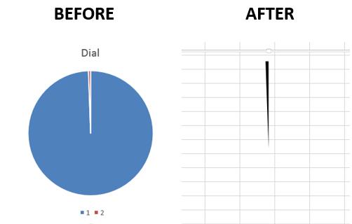
- În panouri Format de serie de date (Format Data Series) change the fill of the larger sector of the chart to Fără umplere (No Fill) and border on no border (No Border).
- Select the small section of the chart that will act as the arrow and change the border to no border (No Border). If you want to change the color of the arrow, select the option umplutură solidă (Solid Fill) and suitable color.
- Click on the background of the chart area and in the panel that appears, change the fill to Fără umplere (Fără umplere).
- Click the sign icon la care se adauga (+) for quick menu access Elementele diagramei (Chart Elements) and uncheck the boxes next to Legendă (Legend) и Nume si Prenume (Titlul diagramei).
- Next, place the hand above the dial and rotate it to the desired position using the parameter Unghiul de rotație al primului sector (Angle of First Slice).
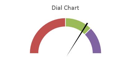
Ready! We just created a watch face chart!