Cum să înghețe mai multe coloane în Excel

The ability to freeze columns in Excel is a useful feature in the program that allows you to freeze an area to keep information visible. It is useful when working with large tables, for example, when you need to make comparisons. It is possible to freeze a single column or capture several at once, which we will discuss in more detail below.

How to freeze the first column in Excel?

To freeze a lone column, you need to do the following:

1. Open the table file you want to edit.
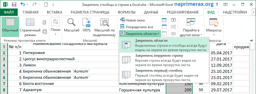
2. Go to the toolbar in the “View” section.
3. Find in the proposed functionality “Lock areas”.
4. In the drop-down list, select “Freeze first column”.

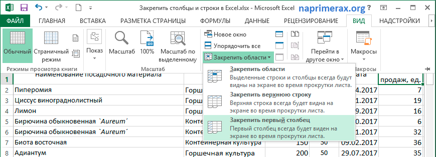
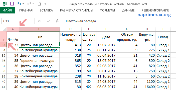
After completing the steps, you will see that the border has changed a little, become darker and a little thicker, which means that it is fixed, and when studying the table, the information of the first column will not disappear and, in fact, will be visually fixed.

How to freeze multiple columns in Excel?

To fix several columns at once, you have to perform a number of additional steps. The main thing to remember is that the columns are counted from the leftmost sample, starting with A. Therefore, it will not be possible to freeze several different columns somewhere in the middle of the table. So, to implement this functionality, you need to do the following:

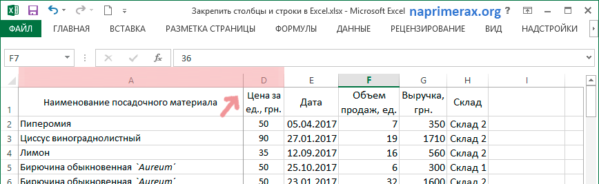
1. Let’s say we need to freeze three columns at once (designations A, B, C), so first select the entire column D or cell D

2. After that, you need to go to the toolbar and select the tab called “View”.
3. In it, you will need to use the option “Freeze areas”.

4. In the list you will have several functions, among them you will need to select “Freeze areas”.
5. If everything is done correctly, then the three indicated columns will be fixed and can be used as a source of information or comparison.

Fii atent! You only need to freeze columns if they are visible on the screen. If they are hidden or go beyond visual visibility, then the fixing procedure is unlikely to end successfully. Therefore, when performing all actions, you should be extremely careful and try not to make mistakes.

How to freeze column and row at the same time?

There may be such a situation that you need to freeze a column at once along with the nearest row, in order to implement a freeze, you need to do the following:

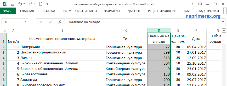
1. At first, you will need to use the cell as the base point. The main requirement in this case is that the cell must be located strictly at the intersection of the row and column. At first, this may sound complicated, but thanks to the attached screenshot, you can immediately understand the intricacies of this moment.
2. Go to the toolbar and use the “View” tab.
3. In it you need to find the item “Freeze areas” and click on it with the left mouse button.
4. From the drop-down list, just select the option “Freeze areas”.

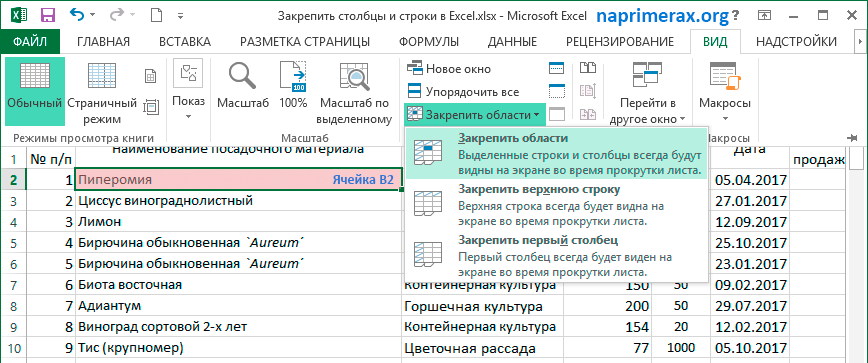
It is possible to fix several panels at once for further use. For example, if you need to fix the first two columns and two lines, then for a clear orientation you will need to select cell C3. And if you need to fix three rows and three columns at once, for this you will need to select cell D4 already. And if you need a non-standard set, for example, two rows and three columns, then you will need to select cell D3 to fix it. Drawing parallels, you can see the principle of fixing and boldly use it in any table.

How to unfreeze regions in Excel?

After the information from the pinned columns is fully used, you should think about how to remove the pinning. There is a separate function specifically for this case, and to use it, you need to do the following:

1. The first step is to make sure that pinned columns are no longer needed for your work.
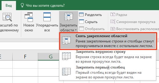
2. Now go to the toolbar at the top and go to the “View” tab.
3. Use the Freeze Regions feature.
4. From the drop-down list, select the “Unfreeze regions” item.

As soon as everything is done, the pinning will be removed, and it will be possible to use the original view of the table again.

Concluzie

As you can see, using the pinning function is not so difficult, it is enough to skillfully apply all available actions and carefully follow the recommendations. This function is sure to come in handy, so you should remember the principle of its use.