


Cuprins
This lesson explains how to quickly deal with a situation where a function VPR (VLOOKUP) does not want to work in Excel 2013, 2010, 2007 and 2003, and how to identify and fix common errors and overcome limitations VPR.
In several previous articles, we have explored the various facets of the function VPR in Excel. If you have read them carefully, you should now be an expert in this field. However, it is not without reason that many Excel experts believe VPR one of the more complex features. It has a bunch of limitations and features that become the source of many problems and errors.

In this article you will find simple explanations of errors #LA (#N/A), #NAME? (#NAME?) and #VALOARE! (#VALUE!) that appear when working with the function VPR, as well as techniques and methods of dealing with them. We’ll start with the most common cases and the most obvious reasons why. VPR does not work, so it is better to study the examples in the order in which they are given in the article.
Fixing #N/A error in VLOOKUP function in Excel
In formulas with VPR mesaj de eroare #LA (#N/A) means nu sunt disponibile (no data) – appears when Excel cannot find the value you are looking for. This can happen for several reasons.
1. The desired value is misspelled
Good idea to check this item first! Typos often occur when you work with very large amounts of data, consisting of thousands of lines, or when the value you are looking for is written into a formula.
2. #N/A error when searching for an approximate match with VLOOKUP
If you use a formula with an approximate match search condition, i.e. argument interval_lookup (range_lookup) is TRUE or not specified, your formula may report an error #N / A in two cases:
- The value to look up is less than the smallest value in the array being looked up.
- The search column is not sorted in ascending order.
3. #N/A error when looking for an exact match with VLOOKUP
If you are looking for an exact match, i.e. argument interval_lookup (range_lookup) is FALSE and the exact value was not found, the formula will also report an error #N / A. Learn more about how to search for exact and approximate matches with a function VPR.
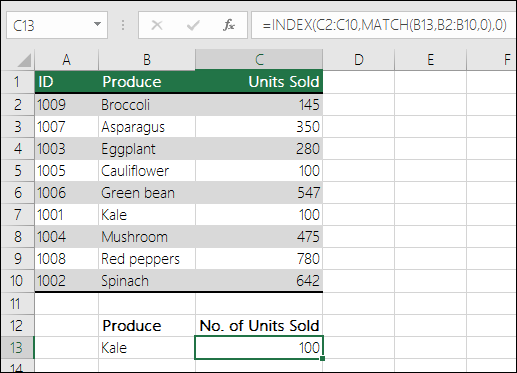
4. Search column is not leftmost
As you probably know, one of the most significant limitations VPR it’s that it can’t face to the left, hence the lookup column in your table must be leftmost. In practice, we often forget about this, which leads to a non-working formula and an error. #N / A.
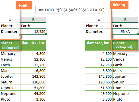
Decizie: If it is not possible to change the data structure so that the search column is leftmost, you can use a combination of functions INDEX (INDEX) și MAI EXPUSĂ (MATCH) as a more flexible alternative for VPR.
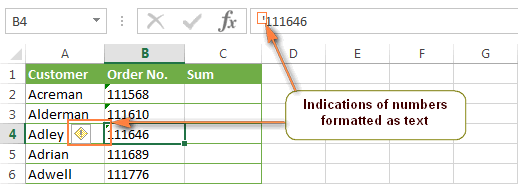
5. Numbers are formatted as text
Another source of error #N / A in formulas with VPR are numbers in text format in the main table or lookup table.
This usually happens when you import information from external databases, or when you type an apostrophe before a number to keep the leading zero.
The most obvious signs of a number in text format are shown in the figure below:
In addition, numbers can be stored in the format General (General). In this case, there is only one noticeable feature – the numbers are aligned to the left edge of the cell, while by default they are aligned to the right edge.
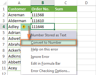
Decizie: If it’s a single value, just click on the error icon and select Convertiți în număr (Convert to Number) from the context menu.
If this is the situation with many numbers, select them and right-click on the selected area. In the context menu that appears, select Celule de format (Format Cells) > tab Număr (Number) > format Număr (Numeric) and press OK.
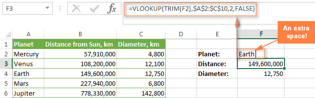
6. There is a space at the beginning or at the end
This is the least obvious reason for the error. #N / A in function VPR, since it is visually difficult to see these extra spaces, especially when working with large tables, when most of the data is off-screen.
Solution 1: Extra spaces in the main table (where the VLOOKUP function is)
If extra spaces appear in the main table, you can ensure that the formulas work correctly by enclosing the argument lookup_value (lookup_value) into a function TUNDE (TUNDE):
=VLOOKUP(TRIM($F2),$A$2:$C$10,3,FALSE)
=ВПР(СЖПРОБЕЛЫ($F2);$A$2:$C$10;3;ЛОЖЬ)
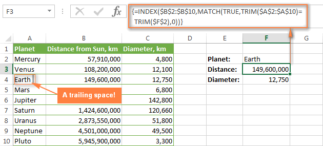
Solution 2: Extra spaces in the lookup table (in the lookup column)
If extra spaces are in the search column – simple ways #N / A în formula cu VPR can’t be avoided. Instead of VPR You can use an array formula with a combination of functions INDEX (INDEX), MAI EXPUSĂ (MATCH) и TUNDE (TUNDE):
=INDEX($C$2:$C$10,MATCH(TRUE,TRIM($A$2:$A$10)=TRIM($F$2),0))
=ИНДЕКС($C$2:$C$10;ПОИСКПОЗ(ИСТИНА;СЖПРОБЕЛЫ($A$2:$A$10)=СЖПРОБЕЛЫ($F$2);0))
Since this is an array formula, don’t forget to press Ctrl + Shift + Enter în loc de obicei Intrațito enter the formula correctly.
Error #VALUE! in formulas with VLOOKUP
In most cases, Microsoft Excel reports an error #VALOARE! (#VALUE!) when the value used in the formula does not match the data type. Concerning VPR, then there are usually two reasons for the error #VALOARE!.
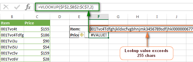
1. The value you are looking for is longer than 255 characters
Be careful: function VPR cannot search for values containing more than 255 characters. If the value you are looking for exceeds this limit, you will receive an error message. #VALOARE!.
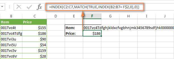
Decizie: Use a bunch of features INDEX+MATCH (INDEX + MATCH). Below is a formula that will do just fine for this task:
=INDEX(C2:C7,MATCH(TRUE,INDEX(B2:B7=F$2,0),0))
=ИНДЕКС(C2:C7;ПОИСКПОЗ(ИСТИНА;ИНДЕКС(B2:B7=F$2;0);0))
2. The full path to the search workbook is not specified
If you are retrieving data from another workbook, you must specify the full path to that file. More specifically, you must include the workbook name (including the extension) in square brackets [ ], followed by the sheet name, followed by an exclamation point. All this construction must be enclosed in apostrophes, in case the book or sheet name contains spaces.
Here is the complete structure of the function VPR to search in another book:
=VLOOKUP(lookup_value,'[workbook name]sheet name'!table_array, col_index_num,FALSE)
=ВПР(искомое_значение;'[имя_книги]имя_листа'!таблица;номер_столбца;ЛОЖЬ)
The real formula might look like this:
=VLOOKUP($A$2,'[New Prices.xls]Sheet1'!$B:$D,3,FALSE)
=ВПР($A$2;'[New Prices.xls]Sheet1'!$B:$D;3;ЛОЖЬ)
This formula will look up the cell value A2 într-o coloană B pe foaie Sheet1 in the workbook New Prices and extract the corresponding value from the column D.
If any part of the table path is omitted, your function VPR will not work and will report an error #VALOARE! (even if the workbook with the lookup table is currently open).
Pentru mai multe informații despre funcție VPRreferencing another Excel file, see the lesson: Searching another workbook using VLOOKUP.
3. Argument Column_num is less than 1
It’s hard to imagine a situation where someone enters a value less than 1to indicate the column from which to extract the value. Although it is possible if the value of this argument is calculated by another Excel function nested within VPR.
So, if it happens that the argument col_index_num (număr_coloană) mai mic decât 1funcţie VPR will also report an error #VALOARE!.
Dacă argumentul col_index_num (column_number) is greater than the number of columns in the given array, VPR va raporta o eroare #REF! (#SSIL!).
Error #NAME? in VLOOKUP
The simplest case is a mistake #NAME? (#NAME?) – will appear if you accidentally write a function name with an error.
The solution is obvious – check your spelling!
VLOOKUP does not work (limitations, caveats and decisions)
In addition to the rather complicated syntax, VPR has more limitations than any other Excel function. Because of these limitations, seemingly simple formulas with VPR often lead to unexpected results. Below you will find solutions for several common scenarios where VPR este greșit.
1. VLOOKUP is not case sensitive
Funcţie VPR does not distinguish between case and accepts lowercase and uppercase characters as the same. Therefore, if there are several elements in the table that differ only in case, the VLOOKUP function will return the first element found, regardless of case.
Decizie: Use another Excel function that can perform a vertical search (LOOKUP, SUMPRODUCT, INDEX, and MATCH) in combination with CORECTA that distinguishes case. For more details, you can learn from the lesson – 4 ways to make VLOOKUP case-sensitive in Excel.
2. VLOOKUP returns the first value found
După cum știți deja, VPR returns the value from the given column corresponding to the first match found. However, you can have it extract the 2nd, 3rd, 4th, or any other repetition of the value you want. If you need to extract all duplicate values, you will need a combination of functions INDEX (INDEX), CEL MAI PUŢIN (MIC) și LINE (ROW).
3. A column was added or removed to the table
Unfortunately, the formulas VPR stop working every time a new column is added or removed to the lookup table. This happens because the syntax VPR requires you to specify the full range of the search and the specific column number for data extraction. Naturally, both the given range and the column number change when you delete a column or insert a new one.
Decizie: And again functions are in a hurry to help INDEX (INDEX) și MAI EXPUSĂ (MATCH). In the formula INDEX+MATCH You separately define search and retrieval columns, and as a result, you can delete or insert as many columns as you want without worrying about having to update all related search formulas.
4. Cell references are garbled when copying a formula
This heading explains the essence of the problem exhaustively, right?
Decizie: Always use absolute cell references (with the symbol $) on records the range, for example $ A $ 2: $ C $ 100 or $ A: $ C. In the formula bar, you can quickly switch the link type by clicking F4.
VLOOKUP – working with the functions IFERROR and ISERROR
If you don’t want to scare users with error messages #N / A, #VALOARE! or #NAME?, you can show an empty cell or your own message. You can do this by placing VPR into a function DACA EROARE (IFERROR) in Excel 2013, 2010 and 2007 or use a bunch of functions IF+ISERROR (IF+ISERROR) in earlier versions.
VLOOKUP: working with the IFERROR function
Sintaxa funcției DACA EROARE (IFERROR) is simple and speaks for itself:
IFERROR(value,value_if_error)
ЕСЛИОШИБКА(значение;значение_если_ошибка)
That is, for the first argument you insert the value to be checked for an error, and for the second argument you specify what to return if an error is found.
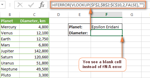
For example, this formula returns an empty cell if the value you are looking for is not found:
=IFERROR(VLOOKUP($F$2,$B$2:$C$10,2,FALSE),"")
=ЕСЛИОШИБКА(ВПР($F$2;$B$2:$C$10;2;ЛОЖЬ);"")
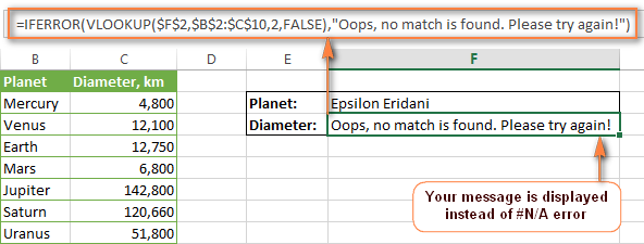
If you want to display your own message instead of the function’s standard error message VPR, put it in quotes, like so:
=IFERROR(VLOOKUP($F$2,$B$2:$C$10,2,FALSE),"Ничего не найдено. Попробуйте еще раз!")
=ЕСЛИОШИБКА(ВПР($F$2;$B$2:$C$10;2;ЛОЖЬ);"Ничего не найдено. Попробуйте еще раз!")
VLOOKUP: working with the ISERROR function
Din moment ce funcţia DACA EROARE appeared in Excel 2007, when working in earlier versions you will have to use the combination IF (IF) and EOSHIBKA (ISERROR) like this:
=IF(ISERROR(VLOOKUP формула),"Ваше сообщение при ошибке",VLOOKUP формула)
=ЕСЛИ(ЕОШИБКА(ВПР формула);"Ваше сообщение при ошибке";ВПР формула)
De exemplu, formula IF+ISERROR+VLOOKUP, similar to the formula IFERROR+VLOOKUPshown above:
=IF(ISERROR(VLOOKUP($F$2,$B$2:$C$10,2,FALSE)),"",VLOOKUP($F$2,$B$2:$C$10,2,FALSE))
=ЕСЛИ(ЕОШИБКА(ВПР($F$2;$B$2:$C$10;2;ЛОЖЬ));"";ВПР($F$2;$B$2:$C$10;2;ЛОЖЬ))
That’s all for today. I hope this short tutorial will help you deal with all possible mistakes. VPR and make your formulas work correctly.